
Baking the (Insight) Cake: Data Modeling for Analysts
At last, the most delicious form of data modeling is here.


In my last two blog posts, we’ve been building an elaborate (and increasingly strained) baking metaphor for how we go from data to insight. We’ve learned about how data engineers are like farmers shipping ingredients to stores and how data and analytics engineers can create standardized packaging for data to make “shopping” for the right data set easier. These two processes are critical to being able to reliably, consistently, and quickly get insights from data that are invisible to outside observers. All eyes are on the last mile: the insights that come from data analysis. Much like baking, your stakeholders are far more interested in getting a piece of your delicious cake than they are in learning about how you picked the ingredients. That being said, if you don’t bake it right you’re liable to make everyone sick.1
“How to develop an insight” could be the basis of an entire book. This blog post is going to be focused on the technical aspects of getting an insight. That being, once you have the question you want to answer and have a rough idea of what data you need, how do you actually assemble the data? Like all phases of the data transformation process, Data Shaping requires data modeling, however, it’s a very different kind of data modeling.
Data Shapes & Level of Detail
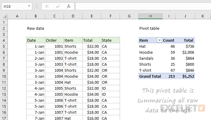
Data Shaping is the final part of the data transformation process and is the most downstream process in a data pipeline. It’s called “shaping” because analysts need to pick a final “shape” for their data to enable analysis. This is done by taking prepared data (hopefully, Tidy Data organized by Data Engineers) and using data modeling techniques to guide the transformation of data into an analytical model. These shapes can take a multitude of different formats, but they are inextricably linked to the kind of technology and the type of analysis you want to do. Some analyses are best done on the raw data itself, while others need to be aggregated up, similar to a pivot table, to better understand what you’re looking at.
The essential first question to ask when shaping a data model for analysis is “What are you counting?” This is a bit more complex than earlier in the pipeline when data engineers work to create atomic tables for each grain. When shaping, your final table is aggregated or grouped based on a specific dimension. So instead of counting observations, you will be counting aggregations of measures across dimensions of interest.
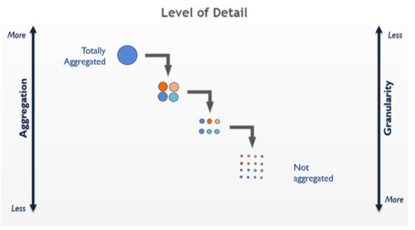
The way I wrapped my head around this was actually early in my career when Tableau was my primary analysis tool. Tableau has an incredibly useful feature called “Level of Detail” expressions that let you operate at multiple levels of aggregation. This image below is basically what I see in my head every time I am trying to aggregate up or down within a data set.
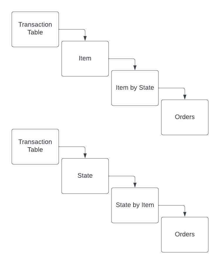
Applying this logic to the above Pivot Table from Excel Jet, you could view the levels of detail for a dataset in two different ways. The first way chooses Item as the primary group, meaning the next level below would be a combination of Item and State. The other way would be using State as the primary group and then a combination of State and Item below that. These end up being the same dataset but for more complex datasets, there are a lot of interesting combinations!
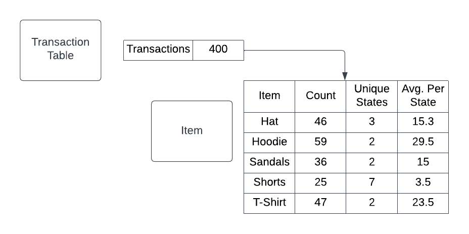
How this actually translates to data is diagrammed below. You can count all the transactions, you can count how many of each item has been sold, you can count how many of each item have been sold by state, and you can look at the individual orders.
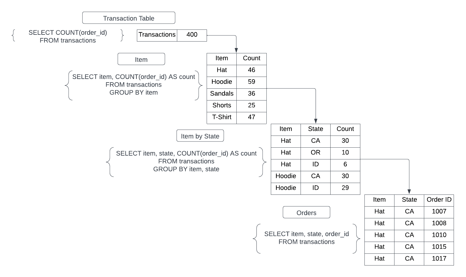
This can lead to some complex Level of Detail questions. For example, if you want to know which item is sold the most on average per state, you’ll need to count the unique State values for each Item aggregation and then divide that by the Count of Items. Ultimately, you are still “counting” the type of Item sold but you will need to look at the underlying data by different levels of detail to get the answer you’re looking for.
Setting Your Kedge
A kedge is a secondary anchor that a ship uses to set the direction that it needs to go. This helps keep the ship on track and move toward its desired destination. The “kedge” metaphor has also been adopted by the speculative futures/strategic foresight study. To them, using a “kedge” is imagining the desired future you want to create and working backward from there. I think this concept is applicable to data shaping because it makes more sense to start with the ideal data set in mind and work backward from there.
For example, let’s select the above table that calculates Avg. Items Sold Per State as our kedge. If our theoretically perfect table existed, we would simply need to SELECT this information from our kedge.
SELECT
	item,
	count,
	unique_states,
	avg_per_state
FROM kedge
Alas, data analysis is not that simple! We can systematically deconstruct the kedge to figure out the best way to calculate each metric. Sometimes, multiple metrics can be calculated from the same source. However, with the above table, each metric is going to need to be constructed with a different intermediary data model.
Our first metric, the count of all items sold, is pretty easy to get.
SELECT item, COUNT(item) AS count
FROM transactions
GROUP BY item
The second metric, unique states that items were sold to, is a little more complicated but still pretty simple when calculated in isolation.
SELECT item, COUNT(DISTINCT state) AS unique_states
FROM transactions
GROUP BY item
Our final metric can only be calculated by bringing these two together. This is where CTEs come in! CTE stands for “Common Table Expressions” and are basically imaginary tables that you create at the top of your SQL statement and treat like a table anywhere below. CTEs are preferable to work with than subqueries or some window functions because they are highly readable. It’s easier to follow the “stream” that creates the final SQL statement this way and allows others to understand and meaningfully collaborate with your code.
WITH item_count AS (
	SELECT item, COUNT(item) AS count
	FROM transactions
	GROUP BY item
),

state_count AS (
	SELECT item, COUNT(DISTINCT state) AS unique_states
	FROM transactions
	GROUP BY item
)

SELECT
	item_count.item,
	item_count.count,
	state_count.unique_states,
	item_count.count / state_count.unique_states AS avg_per_state
FROM item_count
LEFT JOIN state_count ON state_count.item = item_count.item
Look at that! Starting with our kedge allowed us to find the two compositional tables, string them together using CTEs, and create a table that looks exactly like our kedge.2
Combining Ingredients
The above example looked at only one table as a source. Data analysis problems are typically more wide-ranging and touch many different business concepts. This is where Tidy Data becomes important. Similar to bakers keeping each important ingredient on hand, if analysts have a table similar to the above transactions table readily available for every observational unit, assembling and shaping data into an analytical model will be as straightforward a process as following a recipe.
Before we start, it’s important to note that there are 6 main transformations you can make to tidied data to create the right data shape for analysis. These are:
Filter
Remove observations from a table
Aggregate
Combine measures to a denser level of detail using a dimensional grouping
Pivot
Create new dimensions from row values
Mutate
Create new dimensions or measures using existing ones as raw material.
Note that when two measures are combined they create a ‘metric’
Sort
Change the order of the observations in a table based on a key
Join
Combine two or more tables into a single table based on a key
When connecting the dots between your kedge and the source tables, consider which combinations of the 6 transformations you need to make in order to create your kedge. This is how you create your “recipe” to bake your cake.
Consider the below data model for the fictional company “Mike & The Mechanics.” This model shows the final tidied data for the products produced, transactions conducted, the components comprising each product, and the suppliers for each component.
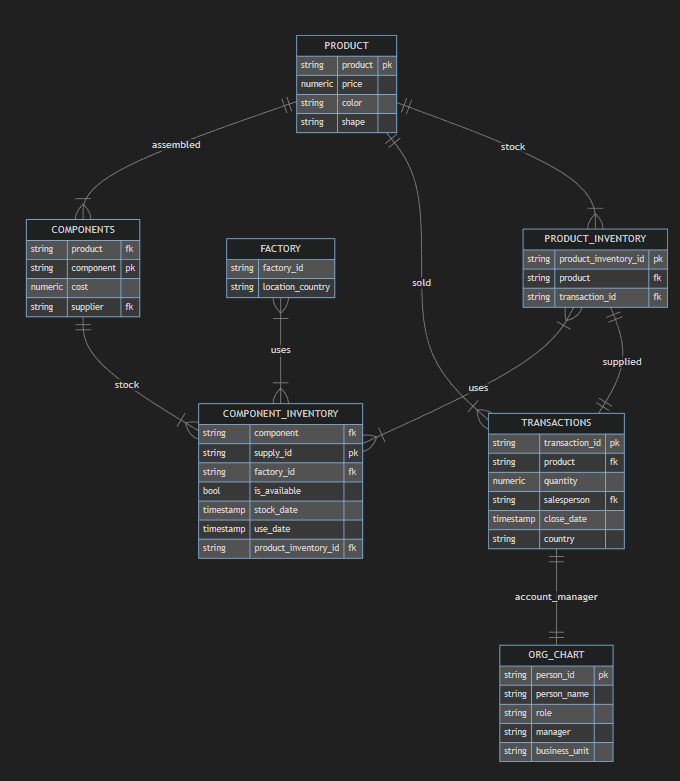
This is a lot closer to what enterprise data looks like (though still quite simplified).
Mike & The Mechanics is a Widgets company headquartered in the United Kingdom but has factories in both France and Spain. It is currently only able to take orders within those 3 countries as well. Mike likes to keep logistics simple and have a product that is sold in a specific country made in that specific country. This isn’t always the case and sometimes Widgets need to be made in different countries and exported to their country of sale. We want to know what countries have the most sales fulfilled by foreign factories and how much revenue those sales represent so Mike can determine if he needs to build an additional factory.
Let’s start with our initial kedge. What do we want our final table to look like so we can perform our analysis?
SELECT

	-- Product Sold by Country
	product,
	sale_country,
	volume_sold,
	revenue_sold,

	-- Product Creation by Country
	domestic_production_rate,
	foreign_production_rate
	domestic_revenue_rate,
	foreign_revenue_rate

FROM kedge
Based on this kedge, the final analytical model is going to require data from the following tables:
PRODUCT (product, price)
TRANSACTIONS (quantity, country, discount)
PRODUCT_INVENTORY (jump table to join other tables)
COMPONENT_INVENTORY (jump table to join other tables)
FACTORY (location_country)
We can draw a simple class diagram to fit the tables above together like puzzle pieces based on their foreign-keys. This will give us a data model that looks like this, where the smallest grain is the component_id. You can determine the smallest grain by following each connection’s multiplicity. The final one-to-many join brings in the component_id.
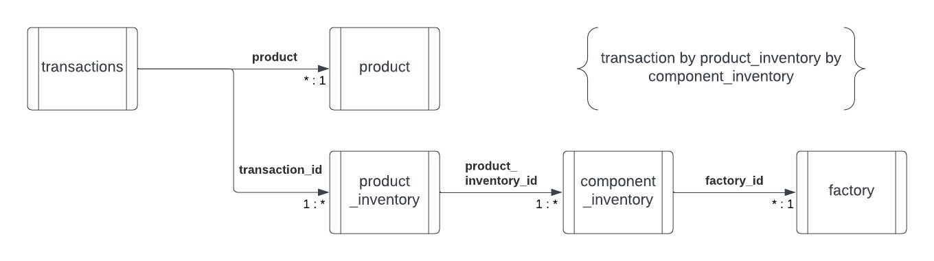
This diagram indicates that we are going to need two branching sets of CTEs to bring together into our final raw table. Let’s first set the kedge for the raw data, so we know what we are developing against.
SELECT
	product,
	price,
	sale_country,
	transaction_id,
	product_inventory_id,
	component_inventory_id,
	production_country
FROM kedge
The first branch of CTEs will transform the TRANSACTIONS table by joining it to the product table.
WITH product_transactions AS (
	SELECT
		product.product,
		product.price,
		transactions.country,
		transactions.transaction_id,
		transactions.product_inventory_id
	FROM product
	LEFT JOIN transactions ON transactions.product = product.product
),
The second branch is going to be more complicated, joining the PRODUCT_INVENTORY, COMPONENT_INVENTORY, and FACTORY tables together.
production_base AS (
	SELECT
		product_inventory.product,
		component_inventory.component_id,
		component_inventory.product_inventory_id,
		factory.location_country AS production_country
	FROM product_inventory
	LEFT JOIN component_inventory ON
		component_inventory.product_inventory_id =
		product_inventory.product_inventory_id
	LEFT JOIN factory ON factory.factory_id =
		component_inventory.factory_id
),
Now we need to join them into one big table from which we can shape our original kedge. We will also want to mutate a new field to help us determine if the product was produced in the same country that it was sold in.
base_join AS (
	SELECT
		product_transactions.product,
		product_transactions.country AS sale_country,
		product_transactions.price,
		product_transactions.transaction_id,
		production_base.component_id,
		production_base.product_inventory_id,
		production_base.production_country AS production_country,
		production_base = production_base.production_country
			AS is_import
	FROM product_transactions
	LEFT JOIN production_base ON
		production_base.product_inventory_id =
		product_transactions.product_inventory_id
),
From here it’s a question of aggregation and mutation to create the final view we want. The first problem we need to deal with was that we only needed the component_inventory table to join in the factory dimension. We can aggregate this data down to the product_id level of detail. Note below that when we GROUP BY every single column we include the price field. This is because price is at the transaction_id level (since we combined it with the product table), not the product_inventory_id level. If we aggregate this measure, we’ll inflate our revenue numbers.
product_grain AS (
	SELECT
		product,
		sale_country,
		price,
		transaction_id,
		product_inventory_id,
		production_country,
		is_import
	FROM base_join
	GROUP BY product, sale_country, price, transaction_id,
		product_inventory_id, production_country, is_import

),
One more aggregation left. Now we want to aggregate at the transaction_id level and mutate a new aggregate field that counts the quantity of distinct product_inventory_ids for each transaction_id.
transaction_grain AS (
	SELECT
		product,
		sale_country,
		price,
		transaction_id,
		COUNT(DISTINCT product_inventory_id) as quantity,
		production_country,
		is_import
	FROM base_join
	GROUP BY product, sale_country, price, transaction_id,
		production_country, is_import

),
With this, we can transform this into our original kedge table through the following steps:
Aggregate volume_sold using quantity on product and sale_country
Mutate two new fields counting domestic volume and foreign_volume based on the value of is_import and aggregate them by product and sale_country
Use the resultant CTE to mutate the following fields:
revenue_sold via multiplying volume_sold times price
production rates by dividing each production volume divided by the total volume sold
revenue rates by multiplying revenue_sold by the production_rates
import_volume AS (
	SELECT
		product,
		sale_country,
		SUM(quantity) AS volume_sold,
		price AS price,
		COUNT(CASE WHEN is_import = True THEN transaction_id END) AS
			domestic_volume,
		COUNT(CASE WHEN is_import = False THEN transaction_id END)
			AS foreign_volume
	FROM transaction_grain
	GROUP BY product, sale_country
),

SELECT
	product,
	sale_country,
	volume_sold,
	(volume_sold * price) AS revenue_sold,
	(domestic_volume / volume_sold) AS domestic_production_rate,
	(foreign_volume / volume_sold) AS foreign_production_rate,
	(volume_sold * price) * (domestic_volume / volume_sold) AS
		domestic_revenue_rate,
	(volume_sold * price) * (foreign_volume / volume_sold) AS
		foreign_revenue_rate
FROM import_volume
There are definitely more “clever” or space efficient ways to develop this analytical model, but the advantage of using this method is that it is highly readable and gives you practice assembling data models formulaically. If your entire team thinks about data similarly, it will be much easier to collaborate on analyses and invite others to give you feedback on your work! Moving forward, if you set your kedges, model your joins, and focus on which combinations of the 6 transformations you need, you’ll be shaping data like a pro in no time.
And if you’d like to see the final SQL all together is one long statement, here you go:
WITH product_transactions AS (
	SELECT
		product.product,
		product.price,
		transactions.country,
		transactions.transaction_id,
		transactions.product_inventory_id
	FROM product
	LEFT JOIN transactions ON transactions.product = product.product
),

production_base AS (
	SELECT
		product_inventory.product,
		component_inventory.component_id,
		component_inventory.product_inventory_id,
		factory.location_country AS production_country
	FROM product_inventory
	LEFT JOIN component_inventory ON
		component_inventory.product_inventory_id =
		product_inventory.product_inventory_id
	LEFT JOIN factory ON factory.factory_id =
		component_inventory.factory_id
),

base_join AS (
	SELECT
		product_transactions.product,
		product_transactions.country AS sale_country,
		product_transactions.price,
		product_transactions.transaction_id,
		production_base.component_id,
		production_base.product_inventory_id,
		production_base.production_country AS production_country,
		production_base = production_base.production_country
			AS is_import
	FROM product_transactions
	LEFT JOIN production_base ON
		production_base.product_inventory_id =
		product_transactions.product_inventory_id
),

product_grain AS (
	SELECT
		product,
		sale_country,
		price,
		transaction_id,
		product_inventory_id,
		production_country,
		is_import
	FROM base_join
	GROUP BY product, sale_country, price, transaction_id,
		product_inventory_id, production_country, is_import

),

transaction_grain AS (
	SELECT
		product,
		sale_country,
		price,
		transaction_id,
		COUNT(DISTINCT product_inventory_id) as quantity,
		production_country,
		is_import
	FROM base_join
	GROUP BY product, sale_country, price, transaction_id,
		production_country, is_import

),

import_volume AS (
	SELECT
		product,
		sale_country,
		SUM(quantity) AS volume_sold,
		price AS price,
		COUNT(CASE WHEN is_import = True THEN transaction_id END) AS
			domestic_volume,
		COUNT(CASE WHEN is_import = False THEN transaction_id END)
			AS foreign_volume
	FROM transaction_grain
	GROUP BY product, sale_country
),

SELECT
	product,
	sale_country,
	volume_sold,
	(volume_sold * price) AS revenue_sold,
	(domestic_volume / volume_sold) AS domestic_production_rate,
	(foreign_volume / volume_sold) AS foreign_production_rate,
	(volume_sold * price) * (domestic_volume / volume_sold) AS
		domestic_revenue_rate,
	(volume_sold * price) * (foreign_volume / volume_sold) AS
		foreign_revenue_rate
FROM import_volume
In Conclusion
I hope I’ve been able to articulate how I view the whole lifecycle of data throughout this series and where data modeling fits in to each phase of the process. Data really can be like baking if you can fill your pantry with ingredients from a fully-stocked grocery store. Much like baking, you can chunk out what you want to create and make each component using easy-to-follow recipes.
I hope you all have many delicious insights in your future!
I have done this both in real life baking and in real life analytics. Don’t do this. This feels bad.
Yes I am aware that there are window functions that you can use to get this same answer. I wanted a simple problem to solve to explain the concept in this blog post.